You've written Python programs that print to the terminal, read files, and maybe even scraped a website. But have you written code that can see? Code that can detect edges in a photograph or find faces in a group picture?
That's computer vision — and it's not as hard to get started as you might think.
OpenCV (Open Source Computer Vision Library) is the tool that makes it possible. Version 5 was announced this June with the biggest set of improvements in years: cleaner Python bindings, named parameters so you're not guessing argument order, and a leaner, faster core. If you're a CS student who knows Python basics, you can be running real computer vision code in under an hour.
What Is OpenCV — and Why Version 5 Matters
OpenCV has been the standard library for computer vision since it was first released by Intel in 2000. It's written in C++ for speed but has Python bindings that make it accessible to anyone. If you've ever used a face unlock on your phone, seen a self-driving car detect pedestrians, or watched a Snapchat filter track your face — there's a good chance OpenCV is somewhere in the pipeline.
Version 5 is a major cleanup release. The OpenCV team stripped out decades of legacy code: the old C API is gone (cvCreateMat() and friends, retired), Python 2 support is dropped (Python 3.6+ only), and the classic machine learning module has been moved to opencv_contrib (the team recommends scikit-learn instead). The Features module got a significant upgrade — renamed from Features2D, it now handles feature vectors from modern deep networks and includes new detectors like ALIKED and DISK, plus the LightGlue feature matcher.
For Python developers, the biggest quality-of-life change is named parameters. In OpenCV 4 you had to remember argument order for every function — cv2.rectangle(img, (x1,y1), (x2,y2), (255,0,0), 2). In OpenCV 5 you can write cv2.rectangle(img, pt1=(x1,y1), pt2=(x2,y2), color=(255,0,0), thickness=2). That alone makes the library far more approachable for beginners.
Under the hood, OpenCV 5 requires C++17, runs a cleaner hardware acceleration layer, and has proper support for FP16/BF16 tensor types. Both the 4.x and 5.x branches are actively maintained, with improvements backported between them — so you're not on a dead-end branch.
Installation — One Line and You're Running
OpenCV 5 was announced on June 4, 2026 with a pip release pending. The command below works with both OpenCV 4.x and 5.x. As of this writing, pip install opencv-python gives you the latest 4.x release (4.13.0.92). Once the 5.0 pip package ships, the same package on PyPI will give you 5.x.
pip install opencv-python
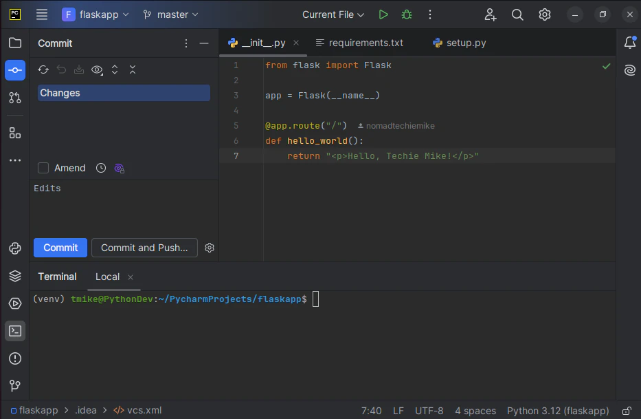
That's it. To verify everything worked, fire up a Python shell:
import cv2
print(cv2.__version__)   # 4.13.x from pip today; 5.x.x once the pip package ships
The code in this guide works with both OpenCV 4.x (from pip) and 5.x (from source). No compilers, no system packages, no fighting with CMake. (If you need the extra modules from opencv_contrib — things like ArUco markers or the xfeatures2d module — install opencv-contrib-python instead.)
For a faster alternative to pip, check out my guide on switching to uv — Python's newer package manager.
I recommend setting up a dedicated virtual environment for your computer vision experiments. If you're not sure how, I've written a full guide on
that walks you through it.
Core Operations — Read, Write, Transform
Every computer vision project starts with the same three steps: load an image, do something to it, save or display the result.
import cv2

# Read an image from disk
img = cv2.imread("photo.jpg")

# Display it (press any key to close)
cv2.imshow("Original", img)
cv2.waitKey(0)

# Save the result
cv2.imwrite("output.jpg", img)
Watch out: OpenCV loads images in BGR format, not RGB. If you pass an OpenCV image to matplotlib or PIL, the colours will look wrong. The fix is a one-liner:
img_rgb = cv2.cvtColor(img, cv2.COLOR_BGR2RGB)
Resize, Crop, and Rotate
These are the three most common transformations — and they're all one or two lines each.
# Resize to a specific width and height
resized = cv2.resize(img, (640, 480))

# Crop — NumPy array slicing. Format: img[y1:y2, x1:x2]
cropped = img[100:400, 200:500]

# Rotate — get the rotation matrix, then apply it
h, w = img.shape[:2]
center = (w // 2, h // 2)
M = cv2.getRotationMatrix2D(center, angle=45, scale=1.0)
rotated = cv2.warpAffine(img, M, (w, h))
Since OpenCV images are NumPy arrays behind the scenes, you can use all your usual NumPy tricks — slicing, stacking, arithmetic — directly on the image data.
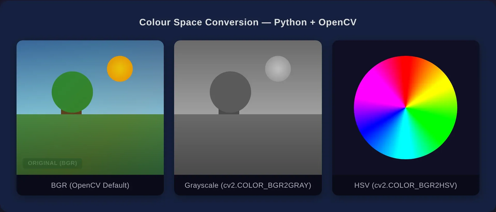
Colour Spaces — RGB, Grayscale, and HSV
Colour space conversion is fundamental to computer vision. OpenCV makes it trivial:
# Grayscale
gray = cv2.cvtColor(img, cv2.COLOR_BGR2GRAY)

# HSV (Hue, Saturation, Value)
hsv = cv2.cvtColor(img, cv2.COLOR_BGR2HSV)
Why does this matter? Grayscale simplifies everything — edge detection, thresholding, and most analysis algorithms work on single-channel images. HSV is useful for colour-based segmentation: isolating objects by colour is far easier in HSV than RGB because the hue channel separates colour from brightness.
If you're studying A-Level Computer Science, this connects directly to the syllabus: image representation (pixels, colour depth, resolution) appears in Paper 1 Theory. For a deeper dive into how computers represent data, check out my

Basic Image Processing — Blur, Detect Edges, Threshold
These three operations form the backbone of most computer vision pipelines. Each is a single function call in OpenCV.
Blurring (Smoothing)
Blurring reduces noise and detail — useful as a pre-processing step before edge detection.
# Gaussian blur — the workhorse
blurred = cv2.GaussianBlur(img, (5, 5), 0)

# Simple averaging blur
blurred_avg = cv2.blur(img, (5, 5))
The (5, 5) is the kernel size — a bigger number means more blur.
Canny Edge Detection
This is the classic algorithm. It finds sharp changes in pixel intensity and draws them as white lines on a black background. Here's the entire pipeline in three lines:
gray = cv2.cvtColor(img, cv2.COLOR_BGR2GRAY)    # Step 1: grayscale
blurred = cv2.GaussianBlur(gray, (5, 5), 0)     # Step 2: smooth
edges = cv2.Canny(blurred, threshold1=50, threshold2=150)  # Step 3: detect
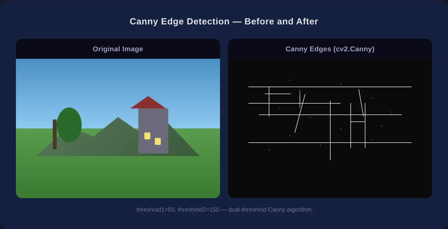
The two thresholds control sensitivity. Any gradient above 150 is definitely an edge. Below 50 is definitely not. Between 50 and 150, it's an edge only if it connects to a strong edge. This dual-threshold approach is what makes Canny so reliable — it catches real edges while ignoring noise.
If you're curious about the underlying maths: Canny computes the image gradient (rate of change) in the x and y directions, finds the magnitude and direction of each gradient, then applies non-maximum suppression to thin the edges. It's a beautifully simple algorithm that's been the standard since 1986.
Thresholding
Thresholding converts a grayscale image to pure black and white based on a cutoff value.
gray = cv2.cvtColor(img, cv2.COLOR_BGR2GRAY)
_, binary = cv2.threshold(gray, thresh=127, maxval=255, type=cv2.THRESH_BINARY)
Every pixel below 127 becomes black (0), every pixel above becomes white (255). This is the simplest form of image segmentation and the foundation for more advanced techniques like adaptive thresholding and Otsu's method.
Drawing Shapes and Text
OpenCV can draw directly onto images — useful for annotating detection results or visualising data.
# Rectangle — perfect for bounding boxes
cv2.rectangle(img, pt1=(50, 50), pt2=(200, 200), color=(0, 255, 0), thickness=2)

# Circle
cv2.circle(img, center=(320, 240), radius=50, color=(0, 0, 255), thickness=-1)  # -1 fills it

# Line
cv2.line(img, pt1=(0, 0), pt2=(640, 480), color=(255, 0, 0), thickness=3)

# Text
cv2.putText(img, text="Hello OpenCV", org=(50, 450),
            fontFace=cv2.FONT_HERSHEY_SIMPLEX, fontScale=1.0,
            color=(255, 255, 255), thickness=2)
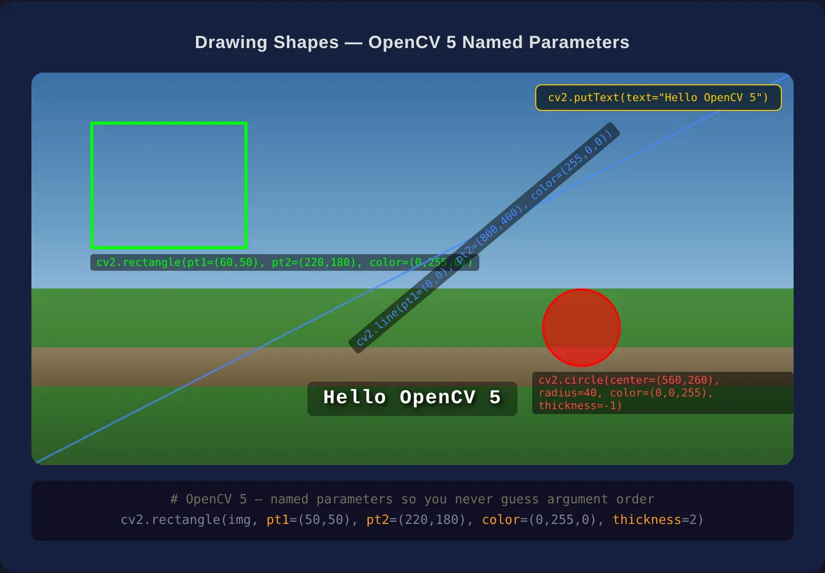
Notice the named parameters — pt1=, color=, thickness= — this is the OpenCV 5 Python improvement at work. No more remembering whether thickness comes before or after the colour tuple.
Mini-Project — Face Detection in 15 Lines
Let's pull everything together with a working face detector. OpenCV ships with pre-trained Haar cascade classifiers — XML files that describe what a frontal face looks like in terms of simple features (edges, lines, rectangles at different scales).
Here's the full script:
import cv2

# Load the pre-trained face cascade
face_cascade = cv2.CascadeClassifier(
    cv2.data.haarcascades + "haarcascade_frontalface_default.xml"
)

# Read the image
img = cv2.imread("group-photo.jpg")
gray = cv2.cvtColor(img, cv2.COLOR_BGR2GRAY)

# Detect faces
faces = face_cascade.detectMultiScale(
    gray, scaleFactor=1.1, minNeighbors=5, minSize=(30, 30)
)

# Draw rectangles around each face
for (x, y, w, h) in faces:
    cv2.rectangle(img, pt1=(x, y), pt2=(x + w, y + h),
                  color=(0, 255, 0), thickness=2)

# Save and display
cv2.imwrite("faces-detected.jpg", img)
print(f"Found {len(faces)} face(s). Output saved.")
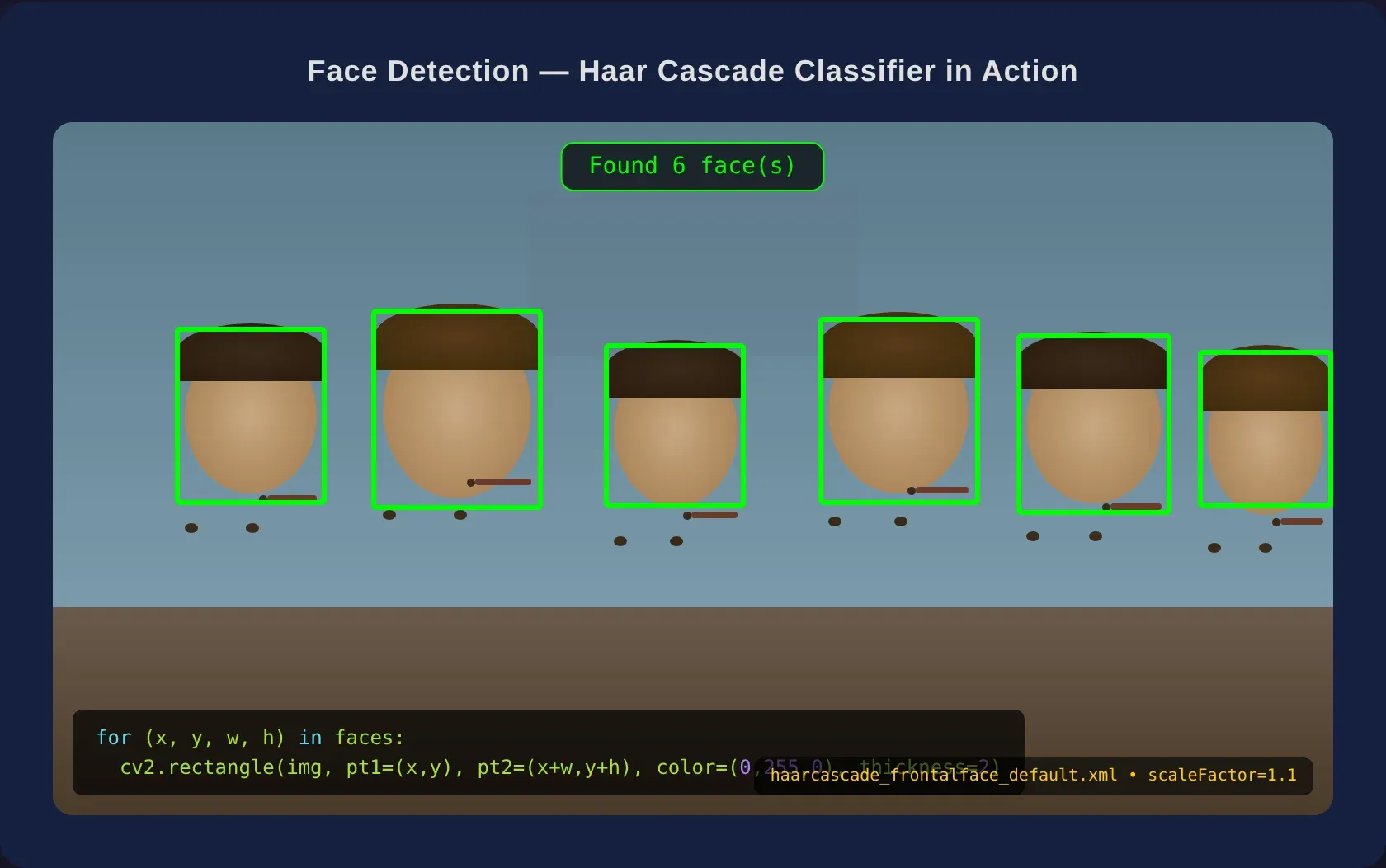
The parameters worth understanding: - scaleFactor=1.1 — the image is scaled down by 10% at each pass. Smaller values (like 1.05) are more accurate but slower. - minNeighbors=5 — how many overlapping detections are needed to confirm a face. Higher values reduce false positives. - minSize=(30, 30) — ignore anything smaller than 30×30 pixels.
Run this on a group photo and you'll get bounding boxes around every face the cascade finds. It's not perfect — Haar cascades are 2001-era technology and can miss faces at odd angles or in poor lighting — but for a 15-line script, the result is impressive.
If you want to try live face detection from a webcam, swap the image loading for a video capture loop:
cap = cv2.VideoCapture(0)  # 0 = default webcam

while True:
    ret, frame = cap.read()
    gray = cv2.cvtColor(frame, cv2.COLOR_BGR2GRAY)
    faces = face_cascade.detectMultiScale(gray, 1.1, 5, minSize=(30, 30))

    for (x, y, w, h) in faces:
        cv2.rectangle(frame, (x, y), (x + w, y + h), (0, 255, 0), 2)

    cv2.imshow("Live Face Detection", frame)
    if cv2.waitKey(1) & 0xFF == ord("q"):
        break

cap.release()
cv2.destroyAllWindows()
Press q to quit. That's real-time computer vision running on your machine.
Where to Go Next
You've covered the fundamentals: loading images, transforming them, detecting edges, and finding faces. From here, OpenCV opens up into a much larger world:
- Object tracking — follow a moving object across video frames with
cv2.TrackerAPIs. - Optical character recognition (OCR) — extract text from images using OpenCV's EAST text detector or pairing OpenCV with Tesseract.
- Feature matching — find the same object in two different images using ORB or SIFT, then use the new LightGlue matcher for better accuracy.
- Deep learning integration — OpenCV's
dnnmodule can load models from TensorFlow, PyTorch, and ONNX. You can run YOLO object detection or image classification directly within OpenCV. - Training your own detector — once you're comfortable with Haar cascades, try training a custom cascade for a specific object (your face, a logo, a particular object).
The official OpenCV Python tutorials at
are excellent, and the opencv/samples/python directory in the GitHub repo contains dozens of working examples — from camera calibration to augmented reality.
If Python debugging is still something you're working on, I've got a guide on
that covers the skills you'll need when your computer vision code doesn't do what you expect.
Computer vision is one of those topics where the theory clicks when you see the output. Reading about edge detection is fine — seeing your own photo turned into crisp white outlines is better. The code examples in this guide are all self-contained; copy them, swap in your own images, and experiment. Change the thresholds and kernel sizes. Try different cascade files. The fastest way to learn OpenCV is to break things and figure out why they broke.